manga
Go to the manga explore page to try out the recommendations. Note that this page may take some time to load.
See the manga embedding plots page for a visualization of the recommendations through the embedding space.
See the manga feed page for a feed of manga from MangaDex that have been re-ranked.
notes
table of contents
- overview
- embedding overview
- latent semantic indexing (LSI)
- word2vec embeddings
- network embeddings
- approximate nearest neighbors
- evaluation
- personalization
- changelog
overview
We’ve reached the point where we can finally build a reasonable model for making content recommendations. As noted in the groups notes, there are two main recommendation models. The first is collaborative filtering models that rely on implicit user interactions (e.g., favoriting a series). The second class of models is content-based models that rely on properties of the data (e.g., tags, descriptions, etc.). User interaction data is not available through the public API. Instead, we focus on content-based models with the potential for personalization in the future.
We can construct three interesting models with tag data alone. We treat these as baselines for more complex models. These all account for the distributional semantics of tags, but in slightly different ways. The first model is a latent semantic indexing (LSI) model, which uses the singular values of a scaled document-term matrix to project the manga into a low-rank space. We recommend the most similar manga based on the cosine similarity of the left singular vector found by the singular value decomposition (SVD). The second builds on the word2vec model, a neural network that learns to represent words in a vector space. We represent each manga by the average of its tag vectors. Then we use the cosine similarity between manga vectors to make recommendations. The final model makes recommendations based on neighbors in the manga-tag bipartite network. We count all the possible paths between two manga through shared tags to create a manga-manga network. We then recommend the most similar manga based on the number of shared tags. To ensure consistency among models, we embed the network onto a manifold using UMAP with justification on both the adjacency and laplacian matrices.
One immediate extension we can make to these models is to use frequent itemsets as words instead of just tags. In other words, we consider all bi-grams, tri-grams, etc. of tags as words. Another extension is to incorporate the description of each manga into the vector-space models using transformer models. One such method is to take the BERT or GPT-Neo embeddings of the description and append them to the tag embeddings. Finally, we can consider adding in popularity or rating statistics to the models. These statistics would likely act as a bias term to re-rank recommendations, and would likely require hyper-parameter tuning to be effective.
embedding overview
We will talk about embeddings throughout the rest of this page. An embedding is a low-dimensional geometric representation of a high-dimensional space which preserves the relative distances between points. These embeddings are metric spaces defined by their embedding e.g. the Euclidean distance or cosine distance. The Euclidean distance is the most common metric, and is what you would use to measure the distance between two points in a 2D or 3D space. It is also known as the norm, and is defined as:
We might instead be interested in the angle between two points. This is common with very sparse vectors, where each column of the vector might represent a (normalized) count feature. The cosine distance would then reflect the number of common features between two vectors as an angle. The cosine distance is defined as the dot product between two points divided by the product of their norms:
We build embeddings because the low-dimensional vector space is much easier to work with and visualize. Our recommendation models can simply compare the distance between two points in the embedding space to determine how similar they are. We make use of efficient algorithms to find the nearest neighbors to a given point, and can even use the embedding to visualize the data. One example that we go into depth later is embedding a network (or graph) into a smaller vector. There are 64k manga in the dataset; when represented as an adjacency matrix of (64464, 64464) elements of 32-bit floats it takes up 15.5 GiB of memory. We can preserve distances by embedding this into a vector of (64464, 256) elements, which takes up 62 MiB of memory. This is several orders of magnitude smaller, while preserving nearest neighbor relationships from the original space.
distribution of tags
Our embeddings will focus on tag data. These are available for all manga, and is the primary way that users might search for manga. All of the embeddings exploit distributional semantics of tags i.e. the meaning of a tag is determined by the tags that appear near it, and the meaning of a manga is determined by the tags that appear on it.
Here we show a histogram often a given tag appears in the dataset.
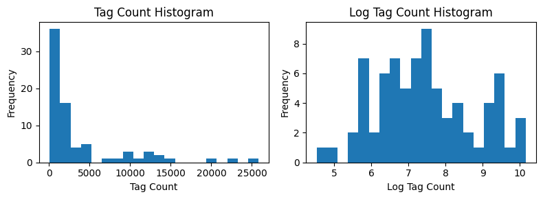
The histogram represents the distribution of tag counts. We note that a few tags appear very frequently, while most tags appear very infrequently. If we take the log of the tag counts, we can see that the distribution looks more like a normal distribution. The raw aggregated data can be found in the following table:
genre
| name | count |
|---|---|
| Romance | 25827 |
| Comedy | 22401 |
| Drama | 19622 |
| Slice of Life | 13781 |
| Fantasy | 12470 |
| Boys’ Love | 11896 |
| Action | 11559 |
| Adventure | 7232 |
| Girls’ Love | 4989 |
| Psychological | 4780 |
| Tragedy | 4103 |
| Mystery | 4103 |
| Historical | 3744 |
| Sci-Fi | 3053 |
| Horror | 2802 |
| Isekai | 2112 |
| Thriller | 1892 |
| Sports | 1600 |
| Crime | 1156 |
| Philosophical | 841 |
| Mecha | 810 |
| Wuxia | 365 |
| Superhero | 359 |
| Medical | 342 |
| Magical Girls | 308 |
theme
| name | count |
|---|---|
| School Life | 13235 |
| Supernatural | 9179 |
| Magic | 2860 |
| Martial Arts | 2453 |
| Harem | 2389 |
| Monsters | 2262 |
| Demons | 1789 |
| Crossdressing | 1762 |
| Survival | 1730 |
| Reincarnation | 1708 |
| Loli | 1670 |
| Office Workers | 1459 |
| Animals | 1444 |
| Military | 1361 |
| Incest | 1238 |
| Shota | 1203 |
| Video Games | 1138 |
| Delinquents | 1081 |
| Monster Girls | 965 |
| Genderswap | 933 |
| Time Travel | 839 |
| Ghosts | 755 |
| Cooking | 755 |
| Police | 712 |
| Vampires | 622 |
| Music | 608 |
| Mafia | 586 |
| Post-Apocalyptic | 546 |
| Aliens | 538 |
| Reverse Harem | 459 |
| Villainess | 415 |
| Gyaru | 362 |
| Samurai | 343 |
| Zombies | 303 |
| Virtual Reality | 226 |
| Ninja | 215 |
| Traditional Games | 133 |
format
| name | count |
|---|---|
| Oneshot | 14874 |
| Doujinshi | 11985 |
| Web Comic | 10328 |
| Full Color | 9369 |
| Long Strip | 9084 |
| Adaptation | 4225 |
| Anthology | 1664 |
| 4-Koma | 1277 |
| Official Colored | 1211 |
| Award Winning | 692 |
| User Created | 531 |
| Fan Colored | 92 |
content
| name | count |
|---|---|
| Sexual Violence | 2103 |
| Gore | 1783 |
We also take a look at how many tags each manga has.
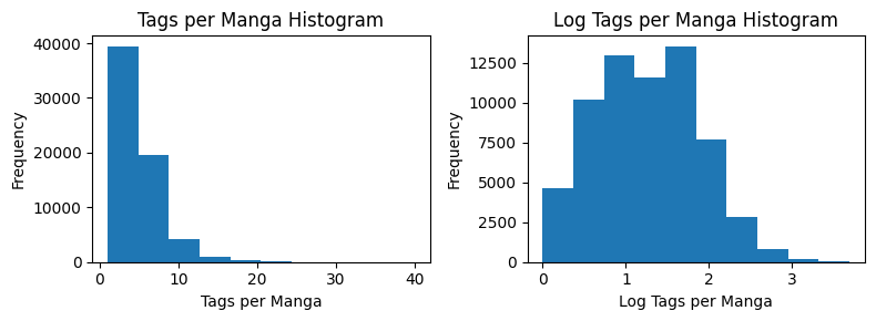
Like before, we note that the distribution is heavy-tailed, and looks more normal when we take the log of the counts.
latent semantic indexing (LSI)
Latent semantic indexing (LSI) a traditional information retrieval technique used to find similar documents based on the frequency of words in the documents. It indexes into a latent (low-rank, probabilistic) space formed by the singular value decomposition (SVD) of a scaled document-term matrix. The LSI recommendation model is theoretically sound, and makes a good baseline for comparison.
document-term matrix and tf-idf
We generate a term-document matrix where each row is a manga, and each column is a tag count. We normalize the tag counts by term frequency-inverse document frequency (tf-idf) to account for the fact that some tags appear more frequently than others. This helps the relevance of tags that occur rarely, but form a coherent cluster in the data. The term frequency is the relative frequency of a term in a document :
The inverse document frequency is a measure of how much information a term provides. If a term appears in more documents, then it is less informative and is therefore down-weighted.
Together, this gives us the tf-idf score:
This is a common weighting scheme that is used in information retrieval systems like Lucene and Elasticsearch.
indexing and querying with SVD
We could use the tf-idf vector representation of terms to find similar manga. However, this representation doesn’t take into account the relationships between terms. We can use the SVD to find a lower-dimensional representation (latent space) of the data that preserves the relationships between terms. This is a type of soft-clustering, where each manga is now represented as a weighted sum of membership in various tag clusters.
SVD decomposes a matrix into a left singular vector, a diagonal matrix of singular values, and a right singular vector.
This is a linear transformation that finds a projection that preserves the largest variance in the data. To make a query into the latent space, we first transform a set of tags into a tf-idf query vector . We then map this query vector into the latent space by multiplying it by the left singular vector .
Then, we just find the nearest neighbors by finding the closest points by cosine distance.
word2vec embeddings
The word2vec model is a neural network that learns to represent words in a vector space. We use the word2vec model to represent tags in a vector space. We represent each manga as an average of its tag vectors, and use the cosine similarity between manga vectors to make recommendations.
There are two methods for training word2vec models: continuous bag of words (CBOW) and skip-gram.
The skip-gram model is order-sensitive, and learns the probability of a word given its context.
This is not ideal for our use case, because tags are not ordered.
The PySpark implementation of word2vec relies on the skip-gram model, so we use gensim to train a CBOW word2vec model on the tag data.
The set of tags on a manga is treated as a sentence in the model.
We set the embedding size to a vector of size 16, which is justified by the square root of the number of tags rounded to the nearest power of 2.
We visualize the tag embeddings using UMAP.
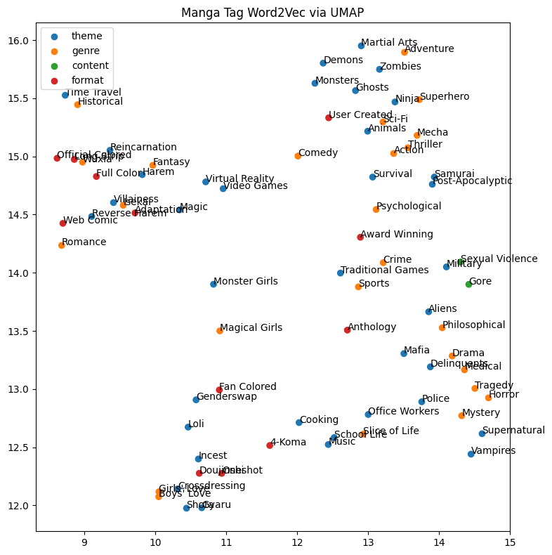
The dimensions are meaningless, but the relative distances between tags are meaningful. We see meaningful clusters of tags, such as “isekai”, “villianess”, “reincarnation”, and “fantasy”.
network embeddings
We can also look at recommendations through a network representation.
construction
We represent our network as matrices. We generate a bipartite adjacency matrix between manga and tags, where each row is a manga, and each column is a tag. We project this matrix into a single mode, to get a manga-manga network where two manga are connected by the dot product of their tags.
There are two representations that interest us: the adjacency matrix and the Laplacian matrix. The adjacency matrix has a row and column for each manga, where two manga are connected by the number of shared tags. The Laplacian matrix is the degree matrix minus the adjacency matrix.
The laplacian matrix is related to connectivity of the graph, and is often used for clustering.
removing indirect effects
We explore two techniques to remove indirect effects from the network, as described by this nature article (scihub link). These techniques were designed for a gene regulatory network inference task, but can be applied to our network. Our network construction is purely indirect, since it relies on paths through tags to connect manga. As we introduce derivative tags representing pairs and triplets of tags, we introduce even more indirect effects. Therefore, it might be interesting to determine the effects of removing indirect effects from the network.
Neither of these methods are tractable on the full 64k manga dataset, but it’d be interesting to try this on a smaller subset of the data in the future.
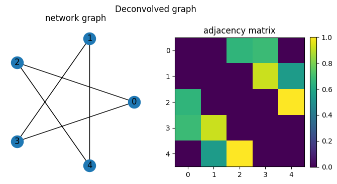
network deconvolution
Network deconvolution is a general method for removing indirect effects from a network. We use the following closed form equation to represent the transitive closure over the network.
The network deconvolution is represented as follows:
Concretely, we perform the following operation, which rescales the eigenvalues found through the eigen decomposition of the adjacency matrix.
def network_deconvolution(G):
    """Deconvolve a network matrix using the eigen decomposition.
    https://www.nature.com/articles/nbt.2635
    """
    # eigen decomposition
    lam, v = scipy.linalg.eigh(G)
    # rescale the eigenvalues
    # also add small value to avoid division by zero
    lam_dir = lam/(1+lam)
    # reconstruct the deconvolved matrix
    G_dir = v @ np.diag(lam_dir) @ v.T

    # remove diagonal, threshold positive values, and rescale in-place
    np.fill_diagonal(G_dir, 0)
    np.maximum(G_dir, 0, out=G_dir)
    G_dir /= np.max(G_dir)

    # NOTE: check reconstruction
    # G_dir = v @ np.diag(lam) @ v.T
    return G_dir
We find that finding the naive implementation using scipy’s eigen decomposition of the adjacency matrix is very slow. We left the deconvolution running for 8 hours and aborted the program due to the intractability. We note that there is an alternative reparameterization that uses gradient descent, but this is out of scale for this experiment.
We can also SVD of the adjacency matrix to find the deconvolution. Instead of rescaling the eigenvectors of the eigen-decomposition, we just find the inverse of the matrix through SVD by inverting the matrix. Both methods have the same big-O complexity of .
Truncating the results of the eigen decomposition or SVD leads to unstable results on small toy examples; the effects of approximating the matrix are uncertain in this case.
global silencing of indirect correlations
Global silencing of indirect correlations is another method for removing indirect effects from a network. The closed form of the silenced network where indirect effects are removed is given by:
where is an operator that sets everything but the diagonal to zero.
This is a closed form solution that can be computed relatively quickly given the inverse of the adjacency matrix. We can use the psuedo-inverse of the adjacency matrix by computing the truncated SVD of the adjacency matrix.
def network_silencing(G):
    """Remove indirect effects using a silencing method.
    https://www.nature.com/articles/nbt.2601
    """
    # svd of G
    u, s, vh = scipy.linalg.svd(G)

    peturb = np.diag((G - np.eye(G.shape[0])) @ G)
    G_dir = (
        (G - np.eye(G.shape[0]) + np.diag(peturb))
        # multiply with pseudo inverse
        @ (u @ np.linalg.pinv(np.diag(s)) @ vh)
    )

    # remove diagonal, threshold positive values, and rescale in-place
    np.fill_diagonal(G_dir, 0)
    np.maximum(G_dir, 0, out=G_dir)
    G_dir /= np.max(G_dir)

    # NOTE: check reconstruction
    # G_dir = u @ np.diag(s) @ vh
    return G_dir
comparisons on toy networks
First we take a look at the network on ring, where weights between successive nodes are 1, and weights between non-successive nodes are inversely weighted by the distance between the nodes (plus some random noise to break symmetry).
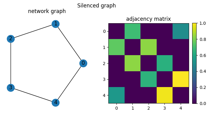
We see that network deconvolution will keep edges with nodes that it shares neighbors with. The network silencing instead removes weak edges in the original network.
The semantics of which method is better depends on the construction of the network.
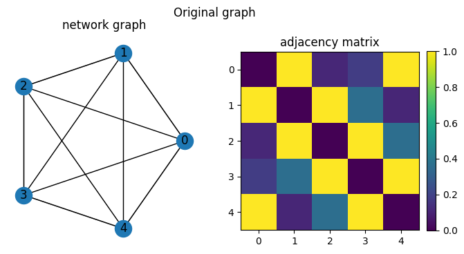
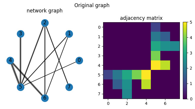
We take a look at another network, which is a bipartite network that we project onto one mode.
We treat the two subsets of nodes and manga and tags, where manga are labeled 0-4 and tags labeled 5-7.
There are node_id % len(tags) edges from each manga to each tag, which are weighted by the originating id of the node.
When we project this, we get a network where each manga is connected to another manga through the number of tags that it shares.
For example, nodes 2 and 4 share two neighbors, so they are connected by an edge that is the dot product of their edge weights.
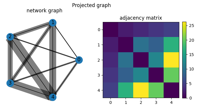
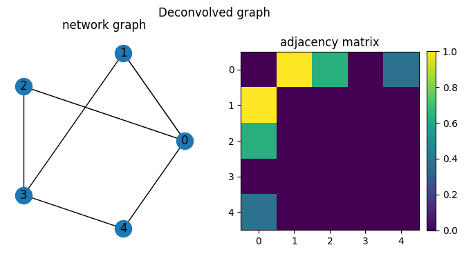
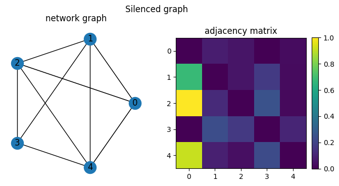
We then run network deconvolution and silencing on the projected network. We note note that the deconvolution method removes edges going through the most common tags, although the behavior is difficult to intuit. The silencing method retains the same structure as the projected network where nodes are connected by edges representing the number of paths between them through tags.
We also note in the context of a fully connected network with equal weights (a clique), the deconvolution method removes all edges while the silencing method retains all edges.
embedding
The spectral embedding model is a method for dimensionality reduction based on network connectivity. We use this to reduce the dimensionality of the network, and to ensure that modeling backends are represented using the same API.
approximate nearest neighbors
We make recommendations by finding the nearest neighbors of each manga in vector space.
nn-descent
NN-Descent is a fast approximate nearest neighbor algorithm that uses a graph to find the nearest neighbors of a point.
pynndescent is an implementation of the algorithm that is suitable for our purposes.
It supports a variety of distance metrics including cosine distances.
locality-sensitive hashing
Locality-sensitive hashing (LSH) is a fast approximate nearest neighbor algorithm that uses a hash function to find the nearest neighbors of a point. LSH is a potential alternative to nn-descent that’s implemented directly in PySpark. However, we are limited to MinHash and Random Projection methods, which only work for Jaccard and Euclidean distances.
evaluation
jaccard index
The Jaccard index is a measure of similarity between two sets. It is defined as follows:
null model
The null model is a baseline for evaluating the performance of a recommendation model. We create a null model by selecting random recommendations for each manga. The null model takes in no information about the data. We then compare the performance through a statistical significance test. We consider using the jaccard R package to perform the tests.
personalization
Personalization is one future direction we could take in developing a recommendation model. We might achieve this by incorporating a weighted average of a query vector with a user’s personalization vector. For example, a user is known to like manga X, Y, and Z. We can represent this preference using the weighted average of tag vectors to form a personalization vector. Then when we query the database for similar manga to a query manga, we also average in user preferences.
changelog
- 2022-12-20: Initial version of the manga recommendations page.
- 2022-12-27: Added reference to network analysis, section on embedding plots
- 2022-12-29: Filling in more of the details for embeddings and some models.
- 2022-12-30: network cleanup work, final embedding plots